9 Validation and science boundaries
9.1 Run the tests
julia --project=. -t auto test/runtests.jl
julia --project=. -t auto scripts/validate.jl --backend=cpu
The first runs tests directly in the active root with its bundled [sources]. The second captures the same run in machine-readable evidence and logs under docs/data. It requires Python 3 in addition to Julia. Do not rely on a Pkg.test() sandbox to inherit active-root path sources. python configuration, units, and reproducible inputs
GPU evidence must be collected on the hardware in its optional environment:
julia --project=environments/metal -t auto scripts/validate.jl --backend=metal
julia --project=environments/cuda -t auto scripts/validate.jl --backend=cuda
Run only the applicable command on a functional device. The underlying GPU gate is scripts/test_gpu.jl --backend=metal|cuda; source inspection or compilation on a device-less host is not an equivalent result.
The results page distinguishes PASS, FAIL, NOT_RUN, and absent evidence. Assertions are checks in a particular suite, not the number of independent scientific experiments or a fractional confidence score.
9.2 What the suites address
| Layer | Test source | What it can establish |
|---|---|---|
| Facade | test/test_configuration.jl |
Configuration validation, units, deterministic options |
| Gravity | test/test_gravity.jl |
Periodic Poisson/particle operators on controlled inputs |
| MHD | test/inherited/runtests.jl |
Exact-wave behavior, conservation/convergence and solver regressions |
| Drag and photons | test/inherited/test_drag_godunov.jl, test_radiation_coupling.jl |
Controlled source response, asymptotic limits, persistent photon fields |
| Species and recombination | test_passive_transport.jl, test_recombination_mixing.jl, test_recombination_transport.jl |
Bounded transport and specified chemistry/reference cases |
| GPU | test/test_backends.jl |
Available backend operators/parity; read actual coverage before generalizing |
| Python | test/python |
Independent reference models, phase/unit contracts, TSV analysis |
test_radiation_coupling.jl test_recombination_transport.jl
An inherited test becomes current evidence only when executed in this extraction. A unit test passing on CPU does not automatically establish GPU correctness or long-run stability. Historical upstream descriptions are useful for planning but their timing and certification numbers are not transplanted.
9.3 Required science matrix
Before publishing a physical UV band or recombination effect:
- Temporal: halve the timestep at fixed ICs and compare at exactly common epochs. Include source cadence, chemistry half-steps and iteration caps, and free-streaming tolerance.
- Spatial: keep the physical cutoff and realization fixed while increasing grid resolution. Compare force spectra as well as magnetic and density fields.
- Spectral: extend cumulative UV bands with identical low-k phases and amplitudes; compare overlap intervals without renormalizing the low band.
- Start redshift: use progressively earlier matched starts at common final epochs. A direct initialized field has no automatically supplied prehistory.
- Chemistry: converge the network, smoothing length, thermal response, table support/interpolation, and hydrogen/helium electron contributions.
- Backend/precision: compare CPU-f32, a CPU-f64 reference where applicable, and the actual GPU. Inspect density/thermal/phase floors, not just total RMS.
- Energy/divergence: report positivity,
divB*dx/Brms, sampled energy changes, and photon perturbation energy with the closure’s unresolved losses. - Restart: compare a continuous trajectory to an equivalent split/resumed run, preserving configuration and source identity.
Choose observable-specific tolerances and signal floors before comparison. RMS agreement alone can conceal phase error, ultraviolet redistribution, wrong clocks, or pressure/tension cancellation.
Define a serialized suite
julia --project=. -t auto scripts/run_suite.jl examples/convergence-suite.toml
# After reviewing its cases and expected cost:
julia --project=. -t auto scripts/run_suite.jl examples/convergence-suite.toml --execute
Without --execute, the suite command validates cases and prints their output locations without evolving them. Cases override tables in a shared base config and run serially when executed, avoiding simultaneous GPU/memory contention. Select a GPU in the base/case run.backend and activate its environment. Validated
The supplied suite is a starting definition, not a completed convergence study. It keeps Gaussian smoothing at the same physical length by using four cells at N64 and eight cells at N128. Review physical wavelength support, projection cadence, and identical output epochs as grids change. Inspect COMPLETED versus STOPPED_AT_LIMIT for every case before comparing histories.
9.4 CFL limit of the unsplit scheme
The :ref integrator is an unsplit 3D MUSCL-Hancock scheme whose predictor uses all three flux directions without transverse corner-transport terms, so its linear stability limit is the classical one for such schemes (about 1/3 in 3D), not 1. The facade therefore rejects run.cfl (and [environment] MHD_CFL) above 0.25 for mhd_solver = "glm" and above 0.30 for "ct" (MAX_STABLE_CFL in src/configuration.jl). cfl is the Courant number of the signal speed smax for CT and of the cleaning speed ch = glm_ch_fac * smax for GLM.
Measured with tools/cfl_stability/cfl_stability.jl (CPU, Float64, periodic 16^3 unless noted, uniform rho = p = 1, an oblique k = (1,2,3) wave plus 1e-6 white noise, plm, hlld, glm_ch_fac = 2; a run is BLOWUP when max|rho-1| reaches 0.1, ok otherwise after the stated steps; the ceiling is bracketed by the largest stable and smallest growing cfl):
| Case | GLM stable / unstable | CT stable / unstable |
|---|---|---|
B = (0.8,0.5,0.4) |
0.26 (4000 steps) / 0.28 (blowup at 1110 steps) | 0.42 (4000 steps) / 0.43 (blowup at 413 steps) |
B = 0, hydro only |
0.32 (3000 steps) / 0.33 (blowup at 1245 steps) | 0.33 (3000 steps) / 0.34 (growth 6.4e3) |
B = 3 (0.8,0.5,0.4) |
0.265 (3000 steps) / 0.27 (blowup) | 0.40 (3000 steps) / 0.45 (growth 1.2e4) |
B as first row, 32^3 |
0.26 (1500 steps) / 0.28 (blowup) | not run |
bulk v = (1,1,1) |
0.26 (3000 steps) / 0.28 (growth 4.5, 2.1 below it) and 0.30 (blowup at 1318 steps) | 0.40 (1500 steps) / 0.50 (blowup) |
The accepted ceilings keep about 6 percent (GLM, 0.25 vs 0.265) and 9 percent (CT, 0.30 vs 0.33) below the lowest stable edge. Raising cfl further does not give a faster valid run: the grid-scale mode grows by more than four orders of magnitude within tens to hundreds of steps. The smoke problems are limited by the cosmological, radiation and particle-displacement caps, not the hydrodynamic CFL, so changing cfl there leaves the step sequence almost unchanged.
9.5 Comparing CT and GLM runs
examples/cosmology-smoke-ct.toml is the CT counterpart of examples/cosmology-smoke.toml; to compare any case, keep the TOML identical except run.mhd_solver, and give each run a new output directory. Expected, documented differences are not discrepancies to fit away:
- The default GLM radiation path projects
Bevery cycle and limits the explicit step bych = glm_ch_fac * smax. CT does neither, so at equalcflits explicit step is the plain CFL step. Whether this matters depends on whether the CFL step or a cosmological/source cap setsdt; the smoke problem is capped bymax_dln_a, where both solvers take identical steps.metadata.tomlrecordsct_step_glm_limited = falseandct_glm_project_every = 0. - CT builds its faces from the initial cell field, which changes that field by O((k dx)^2) near the cutoff. Report the
CT_INITIAL_FACESnumbers (metadata.toml: ct_initial_*). Usingcurl_symbol = "continuum"reduces the change for Batchelor fields. The first history row of a CT run therefore differs from GLM’s at the level of that change, not at Float32 round-off. - Compare actual common redshifts from the
zcolumns, not cycle numbers, and comparedivb_face_dx_over_brms(CT, Float32 round-off) with the centreddivBdx_over_brms(GLM). The centred value of a CT run is not constrained to zero. - Every workflow takes the solver the same way.
run_pmf.jlandrun_suite.jlaccept--mhd-solver=glm|ct(or setrun.mhd_solverper suite case);validate_production.jl --mhd-solver=ct --output=DIRruns the endpoint/restart gate for CT (CT requires--output, so trackeddocs/dataevidence is not touched; its record carriesmhd_solverand the final centred and face divergence);validate_relative_velocities.jl OUT f32 ctruns the controlled velocity checks with CT.scripts/validate.jlruns the solver-agnostic Julia test suite, which contains the CT regressions, so it has no solver flag. - The remaining agreement criteria are those of the science matrix: define tolerances before measuring, and refine timestep and grid separately for each solver. CT runs on the CPU and Metal backends; CUDA is
NOT_RUN.
Matched-pair workflow
examples/ct-vs-glm-suite.toml defines the matched pair (identical except run.mhd_solver) of the smallest cosmology case:
julia --project=. -t auto scripts/run_suite.jl examples/ct-vs-glm-suite.toml          # dry run
julia --project=. -t auto scripts/run_suite.jl examples/ct-vs-glm-suite.toml --execute
uv run pmf-analyze results/ct-vs-glm/glm      # and .../ct
uv run pmf-compare-runs results/ct-vs-glm/glm results/ct-vs-glm/ct
pmf-compare-runs RUN_A RUN_B pairs history.tsv rows and spectra.tsv epochs at common redshifts (--z-tol, absolute, default 1e-3; never by cycle), and reports the relative difference (B - A)/A of every history column and of each spectrum field, plus both divergence diagnostics listed separately (never differenced). Reference values below --floor (default 1e-8) times the column/field-epoch maximum are skipped, not reported as zero: without that floor round-off-level high-k power at 1e-16 dominates the maxima. It writes history_differences.tsv, spectra_differences.tsv, and run_comparison.json and states each run’s solver and status from metadata.toml. It is a difference report, not a gate; tolerances are chosen per the science matrix before measuring.
Terminal and hybrid CT vs GLM
test/inherited/test_terminal_ct_equivalence.jl compares the terminal paths on an ABC-type field (a = 0.08, rho = 1 + 0.02 sin(x+y), gamma_drag = 4, T = 1; periodic unit box; signal S = ||B_glm(T) - B(0)||). Tolerances were fixed before the CT-GLM numbers were computed: d = ||B_ct - B_glm||/S below 0.20 (N=16) and 0.06 (N=32), a ratio d16/d32 above 3, CT face divergence below 1e-12 (Float64) / 1e-5 (Float32) in units of dx/Brms at every step, total-energy bookkeeping at round-off, and Float32/Float64 CT agreement below 1e-3 S. The scheme difference is the edge average of the EMF plus the compact face curl versus the centred cell curl, an O((k dx)^2) symbol difference, hence the 4x fall per doubling. Measured: induction (order 4) 2.74e-2 / 7.43e-3 (ratio 3.69), order 2 2.70e-2 / 7.36e-3, pressure step 2.01e-2 / 5.27e-3, radiation terminal 1.70e-2 / 4.30e-3, first-order velocity steps 1.80e-2 / 4.59e-3; CT divergence 2e-15 (Float64), 1.4e-6 (Float32 induction), 1.4e-7 (Float32 compensated Euler). The hybrid terminal -> handoff -> full MHD comparison satisfies its tolerances (2.6e-2 at N=16 and N=32) but not the pre-declared decrease with N (ratio 1.02, @test_broken): the N=32 GLM Godunov run amplifies a 1e-6 relative momentum perturbation to |dB| = 1.8e-4 (CT: 5.0e-6), so that difference is dominated by noise growth in the GLM reference. The implicit B diffusion has no CPU solver and is checked on Metal only.
9.6 Float32 and thermal floors
The total-energy formulation reconstructs thermal energy by subtracting kinetic and magnetic energy. Float32 cancellation can erase small thermal/chemical perturbations or make floors dominate while the total state remains finite. An internal-energy or temperature curve pinned to a floor is not a converged recombination prediction.
Check p_min, eint_min, temperature_min, all corresponding means/maxima, and sensitivity to MHD_PFLOOR, velocity units, field normalization, timestep, and CPU precision. A larger floor or more diffusive fallback can stabilize a run while changing its science. Record it explicitly.
Guide-field compensated magnetic increments preserve updates below a Float32 field ULP; they do not fix every energy subtraction or photon-density roundoff problem. Tiny density contrasts can be near diagnostic precision even when magnetic divergence is small. Compare complex modes and expected signal size.
9.7 Model limitations
Photon P1. The four evolved photon fields and algebraic stress closure are not a full angular/polarization hierarchy. Tight/free asymptotic agreement does not establish transfer accuracy throughout k*lambda_gamma. Compare matched modes to higher-hierarchy references and converge that reference too.
Lyman-alpha. Gaussian mixing is a smoothing model, not line transport. MHD_CHEM_NONLOCAL_TABLE is an explicitly supplied response table with a finite redshift/wavenumber domain. It requires MHD_CHEM_FALPHA=0 and MHD_CHEM_SMOOTH=local to avoid double-counting. Inspect interpolation and out-of-support behavior. Perturbative tables do not certify strongly nonlinear inhomogeneous recombination. chem_nonlocal_enabled
Thermal sources. Temperature response, subtraction precision, species storage, and the chosen helium/electron model affect recombination and drag. An unchanged average ionization history is not evidence that spatial thermal responses are correct.
Terminal approximations. Terminal/hybrid modes are retained for legacy comparison, require explicit opt-in, and did not earn automatic production status from this extraction. Full-MHD radiation is the public research path.
Reference versus nonlinear solver. Python Schiff/LMHD, photon P1, and Lyman-alpha hierarchy tools are independent controlled models. They do not run the full 3D Julia system. A reference-only handoff, a plotted paper curve, or a matching one-zone history is not a reproduction of all Schiff full-3D results.
9.8 Python reference checks
End-to-end native MHD comparison
uv sync --extra test
uv run pmf-compare-nonlinear results/native-mode-metal --backend=metal \
  --resolution=32 --zend=3190 --outputs=5 --execute
This command executes the actual standalone Julia driver from a correlated photon-P1 handoff. It writes the resolved TOML, production log/tables, comparison.tsv, gate.json, and PDF/PNG overlays. The independent P1 model starts from the actual jointly transferred modes without fitting the evolved amplitudes. The comparison retains physical peculiar velocities and complex phase; reference and production source hashes accompany its gate. def assess test_velocity_and_particle_clocks_are_distinct
The default z=3200 to 3100 interval is a small controlled test. The command above shortens it further for installation verification. Select z=500 and N64 or higher for through-recombination work, then converge CFL, spatial resolution, source history, and optional nonlocal response table. The default uses full local chemistry, including expansion and helium. --response-table supplies the same nonlocal response to all three stages. The reduced oracle’s hydrogen/thermal closure differs from full H/He evolution; early xHII and thermal perturbations remain explicit model comparisons.
The supplied N32 Metal run uses a 300 pG comoving guide field, perturbation fraction 0.025, and a 1 ckpc/h box. Its 45 resolved evolved observables pass the 5% amplitude and 0.03-radian phase gates over z=3200 to 3190; the measured worst errors are 0.0759% and 1.79e-6 radians. The code, solver/reference hashes, and actual configuration are in the gate, complex-mode table, handoff metadata, and run metadata. This short test’s amplitudes are large enough for Float32 comparison. It does not replace a through-recombination spatial/temporal convergence study.
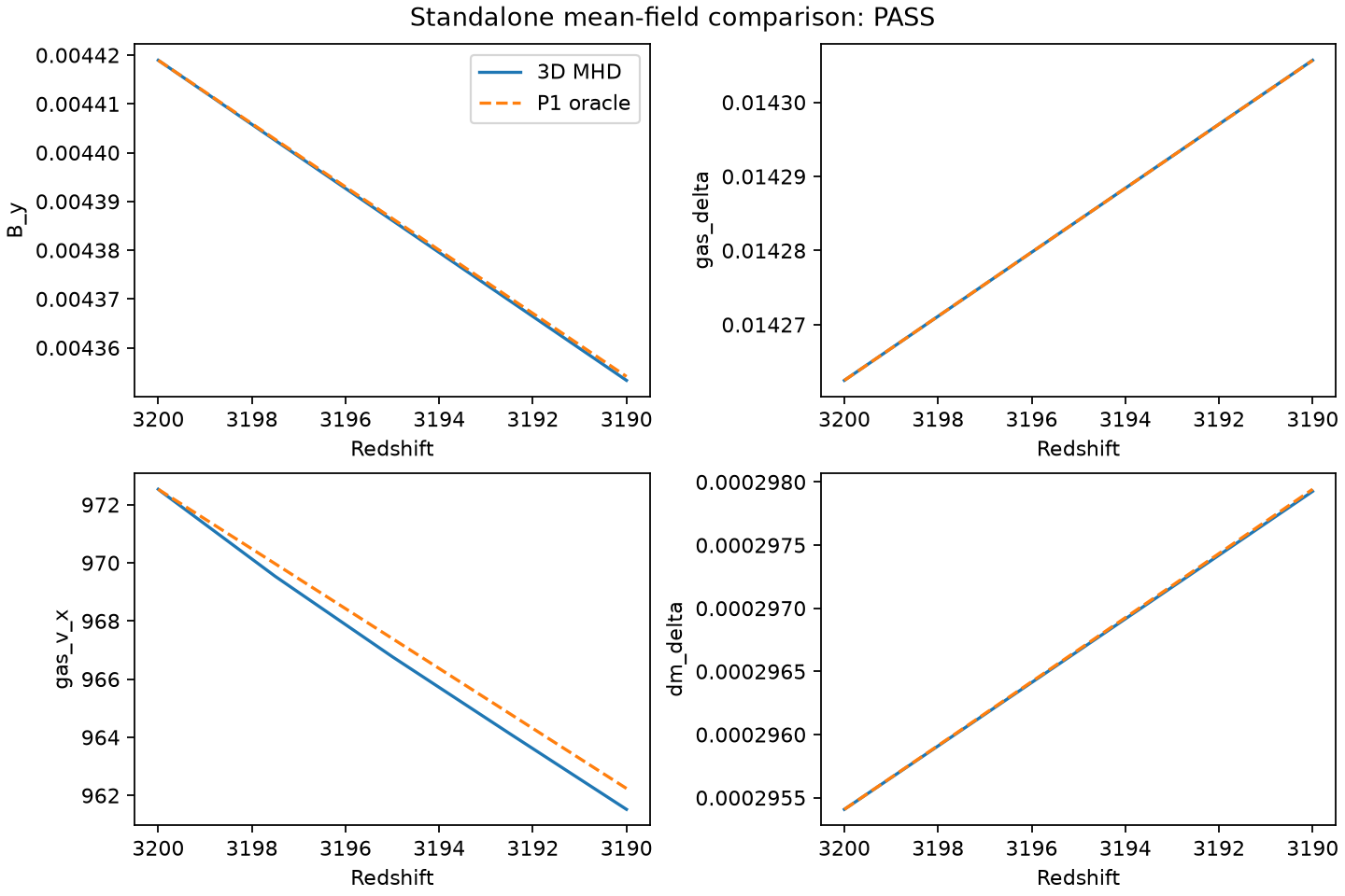
Download the vector comparison figure. The matched threaded-CPU run also passes, with 0.0766% maximum amplitude error: CPU gate and CPU raw comparisons. Both are GLM runs of the same source fingerprint. The same case with --mhd-solver=ct passes on the CPU with 0.0764% and 1.15e-6 radians, and differs from the GLM run by at most 6.9e-5 in relative amplitude and 1.2e-6 radians (pmf-compare-solvers).
Independent small demo
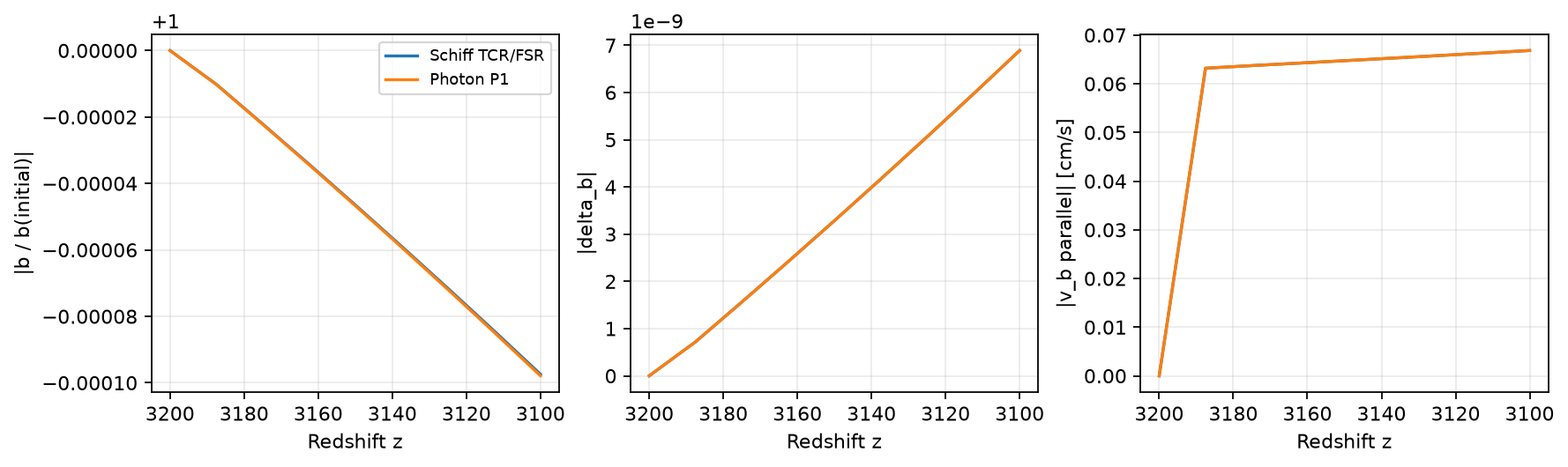
This supplied reference calculation uses k=1000 comoving Mpc^-1 (no h), B0=3e-11 G comoving (30 pG, distinct from the 3 pG Julia example), theta=pi/4, and perturbation fraction 1e-4. Its background is fully ionized hydrogen with no helium electrons, gravity, or evolving baryon-temperature perturbation. The two closures are distinct models, not trajectories required to agree for every mode or epoch. The plotted magnetic axis uses an offset near one; density perturbations here are extremely small.
Reference data and parameters and vector PDF accompany the figure. No conclusion about nonlinear 3D convergence, Lyman-alpha transfer, or GPU parity follows from this demo.
uv sync --extra test
uv run python -m unittest discover -s test/python -v
uv run pmf-reference results/reference
uv run pmf-matched-scenario results/matched
These generate compact reference artifacts and plots. matched_scenario labels its output REFERENCE_ONLY; its NPZ is not a native Julia checkpoint. To compare an evolved candidate, preserve the same complex Fourier convention, units, polarization, epochs, and field names. Read tools/README.md for handoff generators and strict comparison commands. The native nonlinear hierarchy campaign and private/external paper data are not bundled certification.
9.9 Streaming and planar regression scope
The streaming extensions are controlled capabilities, not a completed Tseliakhovich–Hirata cosmological reproduction. The independent matter-era ODE checks exact pressureless growth, transverse-stream invariance, conjugate phases under velocity reversal, and suppression in a declared short-mode example. The shared CPU/device tests check a common physical boost, periodic sampling at moved particles, all three components, and planar MHD invariance. streaming_checks.jl test_streaming.py
The production validator retains its full-physics endpoint smoke and adds a four-cycle planar streaming restart control and sparse/frequent diagnostic comparison. It checks the actual physical-box wavenumber, initial velocity sign and units, and coupled planar invariance with a 5e-6 scaled tolerance. These cycle-limited trajectories are deliberately STOPPED_AT_LIMIT; their restart comparison is not an endpoint or long-time physical convergence result. streaming_initial_check
During this audit, the coupled planar gate exposed a pre-existing diagnostic side effect: inverse-transforming the live photon Fourier state modified its input on FFTW. Diagnostics now copy photon modes to reusable FFT scratch before inversion. Tests assert that photon modes are unchanged by reading maps and that subsequent coherent-flow evolution agrees with a run that did not read them. The production cadence comparison checks this through the coupled driver. photon_fields_to_workspace!
Planar initial conditions still use the full cube, and a constant imposed stream does not generate correlated primordial gas/DM transfer initial conditions. Eulerian relative-velocity spectra with an explicit multistream/empty-cell estimator, a cosmological transfer generator, long-interval matched streaming validation, and a reduced-memory planar coupled backend remain outside this validation scope. Use the streaming conventions and the output workflow when designing a study.